Support Vector Machine Parameters
Welcome to the 33rd part of our machine learning tutorial series and the next part in our Support Vector Machine section. In this tutorial, we're going to be closing out the coverage of the Support Vector Machine by explaining 3+ classification with the SVM as well as going through the parameters for the SVM via Scikit Learn for a bit of a review and to bring you all up to speed with the current methodologies used with the SVM.
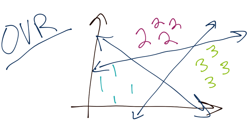
To begin, the SVM, as you have learned, is a binary classifier. This means, at any one time, the SVM optimization is really tasked to separate one group from another. The question is then how we might classify a total of 3 or more groups. Typically, the method is to do what is referred to as "One Verse Rest" or (OVR). The idea here is you separate each group from the rest. For example, to classify three separate groups (1, 2, and 3), you would start by separating 1 from 2 and 3. Then you would separate 2 from 1 and 3. Then finally separate 3 from 1 and 2. There are some issues with this, as things like confidence may be different per classification boundary, also the separation boundaries may be slightly flawed since there are almost always going to be more negatives than positives, since you're maybe comparing one group to three others. Assuming a balanced dataset at the start, this would mean every classification boundary is actually unbalanced.

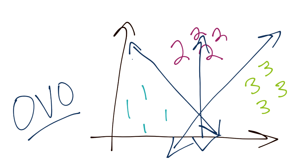
Another method is One-vs-One (or OVO). In this case, consider you have three total groups. The way this works is you have a specific boundary that separates 1 from 3 and 1 from 2, and this process repeats for the rest of the classes. In this way, the boundaries may be more balanced.

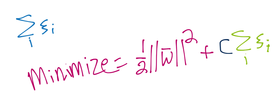
The first parameter is C. This tells you right away that this is a soft-margin classifier. You can adjust C however you like, and you could make C high enough to create a hard-margin classifier. Recall C is used in the soft-margin optimization function for ||w||, like so:

The default value for C is just a simple 1, and that really should be fine in most cases.
Next we have a choice of kernel. The default here is the rbf kernel, but you can also just have a linear kernel, a poly (for polynomial), sigmoid, or even a custom one of your choosing or design.
Next, you have the degree value, defaulting to 3, which is just the degree of the polynomial, if you are using the poly value for the kernel.
gamma is where you can set the gamma value for the rbf kernel. You should leave this as auto.
coef0 allows you to adjust the independent term in your kernel function, but you should also leave this alone most likely, and it is only used in the polynomial and sigmoid kernels.
The probability parameter setting may prove useful to you. Recall how an algorithm like K Nearest Neighbors not only has a model accuracy, but also each prediction can have a degree of "confidence." The SVM doesn't inherently have an attribute like this, but you can use this probability parameter to enable a form of one. This is a costly functionality, but may be important enough to you to enable it, otherwise the default is False.
Next, we have the shrinking boolean, which is defaulted to True. This has to do with whether or not you want a shrinking heuristic used in your optimization of the SVM, which is used in Sequential Minimal Optimization (SMO). You should leave this True, as it should greatly improve your performance, for very little loss in terms of accuracy in most cases.
The tol parameter is a setting for the SVM's tolerance in optimization. Recall that yi(xi.w+b)-1 >= 0. For an SVM to be valid, all values must be greater than or equal to 0, and at least one value on each side needs to be "equal" to 0, which will be your support vectors. Since it is highly unlikely that you will actually get values equal perfectly to 0, you set tolerance to allow a bit of wiggle room. The default tol with Scikit-Learn's SVM is 1e-3, which is 0.001.
The next important parameter is max_iter, which is where you can set a maximum number of iterations for the quadratic programming problem to cycle through to optimize. The default is -1, which means there is no limit.
The decision_function_shape is one-vs-one (ovo) or one-vs-rest (ovr), which is the concept discussed at the beginning of this tutorial.
random_state is used for a seed in the probability estimation, if you wanted to specify it.
Aside from the parameters, we also have a few attributes:
support_ gives you the index values for the support vectors. support_vectors_ are the actual support vectors. n_support_ will tell you how many support vectors you have, which is useful for comparing to your dataset size to determine if you may have some statistical issues. The last 3 parameters dual_coef_, coef_, and intercept_ will be useful if you plan to graph the SVM, for example.
This wraps up the Support Vector Machine. Our next topic is clustering.
There exists 6 quiz/question(s) for this tutorial. for access to these, video downloads, and no ads.
-
Practical Machine Learning Tutorial with Python Introduction
-
Regression - Intro and Data
-
Regression - Features and Labels
-
Regression - Training and Testing
-
Regression - Forecasting and Predicting
-
Pickling and Scaling
-
Regression - Theory and how it works
-
Regression - How to program the Best Fit Slope
-
Regression - How to program the Best Fit Line
-
Regression - R Squared and Coefficient of Determination Theory
-
Regression - How to Program R Squared
-
Creating Sample Data for Testing
-
Classification Intro with K Nearest Neighbors
-
Applying K Nearest Neighbors to Data
-
Euclidean Distance theory
-
Creating a K Nearest Neighbors Classifer from scratch
-
Creating a K Nearest Neighbors Classifer from scratch part 2
-
Testing our K Nearest Neighbors classifier
-
Final thoughts on K Nearest Neighbors
-
Support Vector Machine introduction
-
Vector Basics
-
Support Vector Assertions
-
Support Vector Machine Fundamentals
-
Constraint Optimization with Support Vector Machine
-
Beginning SVM from Scratch in Python
-
Support Vector Machine Optimization in Python
-
Support Vector Machine Optimization in Python part 2
-
Visualization and Predicting with our Custom SVM
-
Kernels Introduction
-
Why Kernels
-
Soft Margin Support Vector Machine
-
Kernels, Soft Margin SVM, and Quadratic Programming with Python and CVXOPT
-
Support Vector Machine Parameters
-
Machine Learning - Clustering Introduction
-
Handling Non-Numerical Data for Machine Learning
-
K-Means with Titanic Dataset
-
K-Means from Scratch in Python
-
Finishing K-Means from Scratch in Python
-
Hierarchical Clustering with Mean Shift Introduction
-
Mean Shift applied to Titanic Dataset
-
Mean Shift algorithm from scratch in Python
-
Dynamically Weighted Bandwidth for Mean Shift
-
Introduction to Neural Networks
-
Installing TensorFlow for Deep Learning - OPTIONAL
-
Introduction to Deep Learning with TensorFlow
-
Deep Learning with TensorFlow - Creating the Neural Network Model
-
Deep Learning with TensorFlow - How the Network will run
-
Deep Learning with our own Data
-
Simple Preprocessing Language Data for Deep Learning
-
Training and Testing on our Data for Deep Learning
-
10K samples compared to 1.6 million samples with Deep Learning
-
How to use CUDA and the GPU Version of Tensorflow for Deep Learning
-
Recurrent Neural Network (RNN) basics and the Long Short Term Memory (LSTM) cell
-
RNN w/ LSTM cell example in TensorFlow and Python
-
Convolutional Neural Network (CNN) basics
-
Convolutional Neural Network CNN with TensorFlow tutorial
-
TFLearn - High Level Abstraction Layer for TensorFlow Tutorial
-
Using a 3D Convolutional Neural Network on medical imaging data (CT Scans) for Kaggle
-
Classifying Cats vs Dogs with a Convolutional Neural Network on Kaggle
-
Using a neural network to solve OpenAI's CartPole balancing environment
